CoreWeave Stock Forecast 2030

In our CRWV Stock Forecast 2030, CoreWeave can become the dominant independent AI cloud and still deliver poor shareholder returns. The size of the platform is close to settled. What remains open is how much value survives the debt, leases, depreciation, and dilution required to build it.

Executive Summary

Walk into a CoreWeave data hall and almost nothing in the room belongs to CoreWeave outright. The building is leased, the racks are financed, and the accelerators inside carry a 6-year accounting life against customer contracts that frequently run shorter. What the company owns is the arrangement itself: the contracts, the software, the deployment competence, and the ability to raise capital against all three faster than anyone else in the sector.

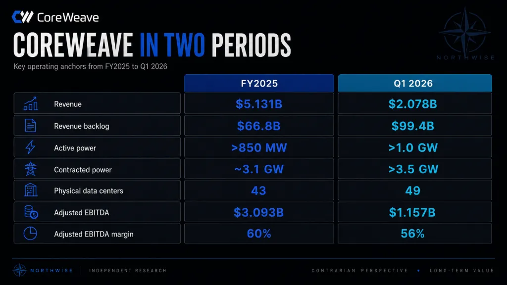
That arrangement has worked spectacularly on the operating side, and the pace is easier to see across two periods than in any single quarter.

Backlog grew by $32.6 billion in a single quarter, and management continues to target more than 8 GW of active power by 2030. The obligations behind that growth expanded on the same schedule. CoreWeave carried $25.1 billion of principal debt at March 31, leases essentially all 49 of its data centers, recognized $10.05 billion of operating lease liabilities, and disclosed a further $40.7 billion of uncommenced lease payments before several construction-linked arrangements.

The market currently values the equity at roughly $39 billion. The backlog is 2.5 times that figure and the contractual lease and debt obligations together exceed it by a wide margin.

Four numbers anchor everything that follows. Our base case reaches 7.5 GW of active power by 2030, averages 6.53 GW of billable capacity across the year, earns a realized fleet density of $14.01 million per billable megawatt, and produces $91.46 billion of revenue. Reaching that point consumes roughly $270 billion of cumulative capital expenditure and carries the diluted share count from 545.6 million to approximately 836 million.

The demand debate is largely settled and the returns debate is not. Nobody serious argues that customers will refuse to sign, since the backlog answers that question directly. The open question is how much of the value created by an enormous, contracted, well-run compute platform actually reaches the residual claimant after landlords, lenders, equipment financiers, convertible holders, and new shareholders take their share.

This forecast is organized in 11 free parts and 5 premium parts. Parts I through III cover what CoreWeave owns, how contracted megawatts become billable ones, and how billable megawatts become revenue. Parts IV through VI cover the cost of building the cloud, why 60% adjusted EBITDA margins can still be expensive, and how the financing stack works in both directions. Parts VII through XI cover competition, the three clocks the thesis runs against, the strongest version of the short case, the variables that move our model, and the complete 2030 operating outcome across four scenarios.

Those four outcomes are worth holding in mind from the start, since every section that follows is an argument about which one CoreWeave lands in.

Notice that revenue varies by a factor of 4 across those rows and free cash flow varies from negative $10.4 billion to positive $47.7 billion. The operating business is considerably more predictable than the shareholder outcome attached to it.

The premium sections then assign a value to each of those four outcomes, weight them, and convert the result into an entry price.

Part I: The Machine

1. What CoreWeave Actually Owns

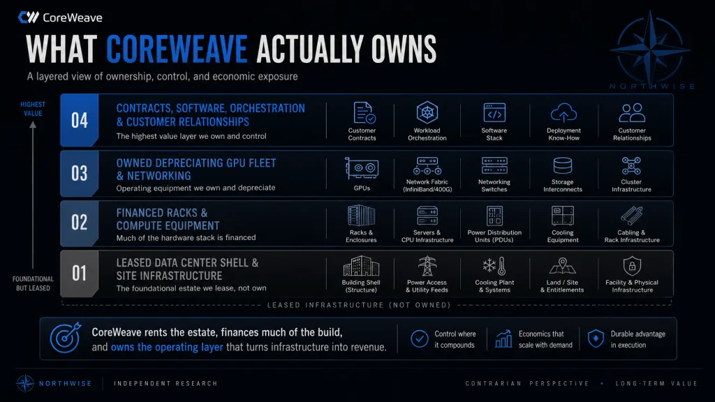
CoreWeave rents almost everything and owns the part that depreciates.

The company operates 49 physical data centers and leases the estate. It buys, finances, installs, and operates the compute inside those buildings, along with the networking fabric, storage, orchestration software, and monitoring systems that turn racks of accelerators into something a customer will pay to use. Revenue comes from selling access to that integrated system under multi-year contracts, mostly to sophisticated buyers who could theoretically build the same thing and have chosen not to wait.

That structure produces an unusual balance sheet. The durable, long-lived, generation-independent layer appears as a lease obligation and the short-lived, rapidly obsolescing layer appears as an owned asset. A landlord holds the substation that will still be useful in 2045, and CoreWeave holds the GPU that will be a mid-tier inference machine in 2032.

The trade buys speed. Leasing lets CoreWeave enter a market without waiting years for grid studies, permitting, and substation procurement, which is precisely why the company reached 1 GW of active power ahead of competitors who own more of their physical footprint. Speed has been worth an enormous amount during a shortage.

What the company genuinely owns is harder to see on a balance sheet. It has an operating record of standing up large multi-node clusters that pass customer benchmarks, a software layer that customers integrate into their production workflows, a procurement relationship with the dominant accelerator vendor, and a financing apparatus that converts signed contracts into project capital at investment-grade terms. Those capabilities are real, and none of them appear as a line item.

2. Ninety-Nine Billion Dollars Does Not Answer the Question

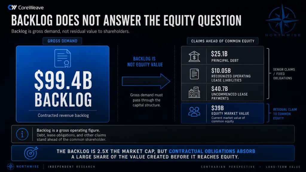
Backlog establishes demand. It says nothing about shareholder returns.

The $99.4 billion figure at March 31 grew from $66.8 billion at the end of 2025, which is an extraordinary rate of commercial accumulation for a company that generated $5.131 billion of revenue in the same prior year. It tells us that large, credit-worthy counterparties want compute at scale, will commit for years, and will sign before the capacity exists. That is the demand question answered as clearly as any company in the sector has answered it.

The question backlog cannot answer is what CoreWeave must spend to deliver it. Every dollar of that $99.4 billion runs through a leased building at contractual rent, on hardware purchased with debt, depreciated across 6 years, and serviced by an organization funded partly through stock-based compensation. The residual after all of that is the only figure that reaches common equity.

A useful way to hold the distinction is to notice that backlog is a gross number on the revenue line and shareholder value is a net number several layers below it. Growth in the first does not automatically produce growth in the second. Our bear case has CoreWeave deliver $59.4 billion of revenue and $30.9 billion of adjusted EBITDA in 2030 while producing roughly nothing for the people who own the stock.

3. The Financing Flywheel

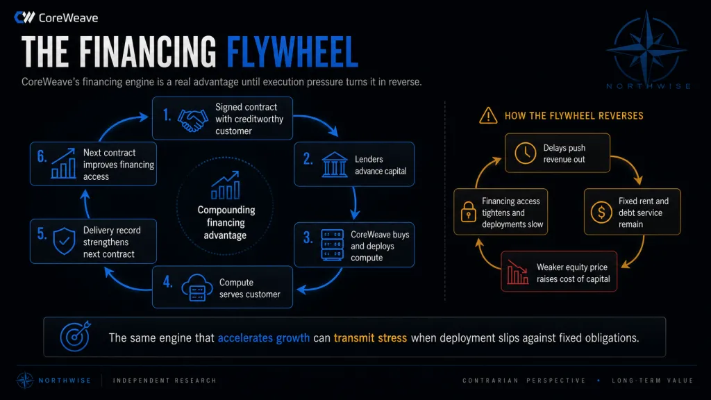
CoreWeave's financing engine is a genuine competitive advantage, and it runs in both directions.

The loop is straightforward. A contract with an investment-grade counterparty gets pledged as collateral, lenders advance capital against the contracted cash flows, that capital buys compute, the compute serves the customer, and the delivery record makes the next contract easier to sign and the next facility cheaper to arrange. The $8.5 billion DDTL 4.0 facility secured in the first quarter of 2026, carrying a floating tranche at SOFR plus 2.25% and a fixed tranche near 5.9%, is the mature version of that machine.

Very few companies can convert a signed contract into deployed capacity this quickly. Competitors with more owned infrastructure move slower on the financing side, and competitors with comparable financing tend to have less operating history to underwrite against. During a period when time to compute is the product, this is close to a moat.

The same mechanism transmits stress with equal efficiency. Delayed capacity means delayed revenue against fixed rent and fixed debt service, which pressures the equity price, which raises the cost of the next dollar of capital, which slows the next deployment. Nothing about the flywheel requires demand to weaken for it to reverse.

Part II: The Physical Build

4. One Megawatt Is Four Different Numbers

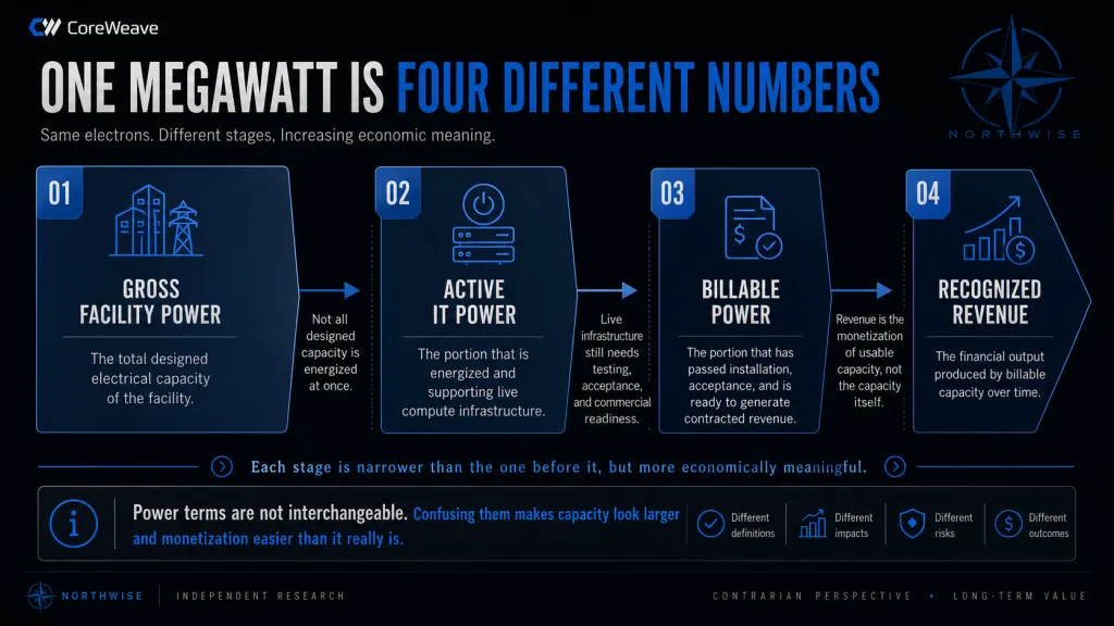
The single most common error in neocloud analysis is treating all megawatts as interchangeable.

The chain runs from utility or gross facility power, to active IT power, to billable power, to recognized revenue. Gross power runs the compute plus the cooling, pumps, fans, lighting, security, and electrical losses that keep it alive. Active IT power is what the compute can actually draw.

Billable power is what a customer has accepted and is paying for. Recognized revenue is what the income statement takes for the period, which depends heavily on when in the year each block came online.

Applying a revenue figure calculated on one basis to a cost figure calculated on another moves project economics by a wide margin in whichever direction the modeler prefers. Our model tracks the schedules separately and never blends them.

One structural point governs the starting position. Active power sits inside contracted power rather than beside it, so the 3.5 GW of contracted capacity at March 31 already includes the 1.0 GW that was active.

The remaining 2.5 GW is the deployment pool CoreWeave draws from before any new contract is required.

5. Reconstructing the 3.5 GW Contracted Estate

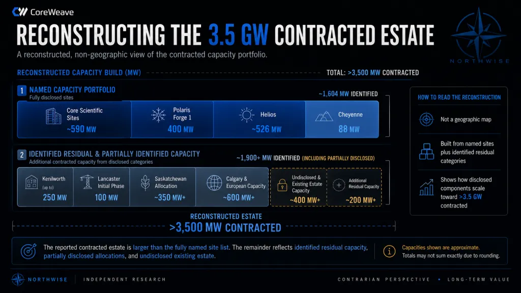
A contracted-capacity figure is only as credible as the sites behind it, so we rebuilt the estate from named assets first.

Beyond that, identified or partially identified capacity includes Kenilworth at up to 250 MW, the Lancaster initial phase at 100 MW, a Saskatchewan allocation, Calgary and European capacity, and additional existing-estate and undisclosed sites. Roughly 1.6 GW of the 3.5 GW is nameable today, and the identified residual accounts for a substantial share of the remainder.

The opening pool therefore does not depend on one enormous unidentified plug. That distinction separates a contracted number that can be underwritten from one that has to be taken on faith.

6. The 2026 and 2027 Bridges

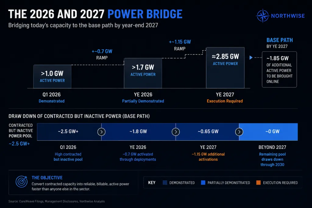
Management guidance constrains the first 2 forecast years tightly enough that scenario dispersion has to come from later cohorts.

For 2026, the company guides to $12 billion to $13 billion of revenue, more than 1.7 GW of year-end active power, and roughly $18 billion to $19 billion of annualized exit revenue. For 2027 it points to more than $30 billion of exit revenue. Our model uses those anchors directly and does not manufacture a dramatically different 2026 simply to widen the distribution.

The 2026 bridge requires roughly 0.7 GW of net additions from the March quarter, against a starting 2.5 GW pool of contracted-but-inactive capacity and 260 MW added during the fourth quarter of 2025 alone. That pace is demonstrated, not hypothetical.

The 2027 bridge to 2.85 GW requires approximately 1.15 GW of additions, which draws down the remaining identified pool and begins to require new contract cohorts entering construction. The 2027 number is where guidance stops doing the work and the model starts.

7. From 3.5 GW Contracted to 7.5 GW Active

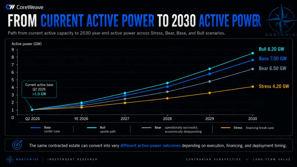
Reaching a 7.5 GW base case requires roughly 4 GW of capacity that has not yet been contracted, which is the central physical assumption in this forecast.

The annual additions behind those totals show where the scenarios separate.

The 2030 row is the one that looks odd on first reading, with bear adding the same 1.60 GW as base. That reflects projects delayed out of earlier years landing late in the forecast period while base has already decelerated into its terminal target. Bear is not building faster in 2030; it is finishing what it should have finished in 2028.

Management's stated ambition of more than 8 GW lives in bull, not base. Base reaches 7.5 GW, which is a large discount to the target and still one of the largest independent compute platforms in the world. Bear reaches 6.5 GW, which is not a failure of the build at all.

Stress assumes substantial project completion before the independent financing model stops working. Even in the scenario where the capital structure has to be reorganized, roughly 4.2 GW gets built, since the capital was committed and the buildings were leased long before the trouble arrived.

8. The Landlord Problem

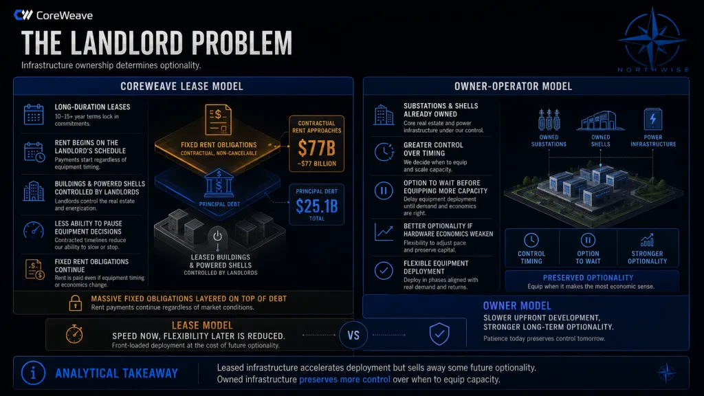
Every operator in this sector faces the same question at the moment hardware economics deteriorate: how expensive is it to stop?

An owner-operator with a completed substation and an unequipped shell can simply wait. The substation holds value across several hardware generations, the land appreciates, and the decision to install compute can be deferred until pricing, prepayments, or a new architecture justify it. That deferral is worth real money, and it is one of the strongest features of the owned-infrastructure model.

CoreWeave typically begins with a long-duration lease. Rent starts on a schedule set by the landlord's delivery, not by CoreWeave's judgment about the return on the next tranche of accelerators. A leased hall that sits partly equipped still generates the full rent obligation, which converts a flexible capital-allocation decision into a fixed cost.

The scale of that commitment is visible in the disclosures. The March 2026 filing showed $16.98 billion of undiscounted commenced operating lease payments and $40.7 billion of uncommenced payments, alongside a separate 525 MW site carrying $18.7 billion to $19.6 billion of contractual rent over 16 years. Total contractual rent therefore approaches $77 billion against $25.1 billion of principal debt.

That last comparison deserves to sit for a moment. CoreWeave's largest long-duration fixed obligation is not its debt.

The trade is coherent rather than careless. Leasing bought the company several years of expansion speed during the precise window when speed was worth the most, and a company that had insisted on owning its estate would have far less active power today. The cost of that choice arrives later, in the form of a weaker stop option exactly when the ability to stop becomes valuable.

Part III: Turning Power Into Revenue

9. Active Does Not Mean Billable

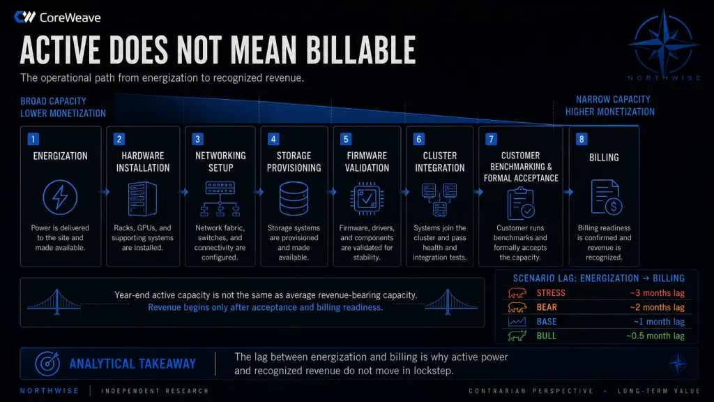
A megawatt that draws power is not a megawatt that bills.

Between energization and the first invoice sit hardware installation, network fabric configuration, storage provisioning, firmware validation, cluster integration, customer benchmarking, and formal acceptance. A cluster spanning thousands of accelerators performs at the level of its weakest layer, and training workloads expose that layer within days. Problems that never appeared during construction surface here, at the point where most of the project capital is already spent.

Our model applies an active-to-billable lag that varies with execution quality: roughly 3 months in stress, 2 months in bear, 1 month in base, and half a month in bull. The differences look small annually and compound significantly across a fleet adding more than a gigawatt a year.

Revenue then attaches to average billable capacity across the year, never to the December figure.

Stress uses 3.520 GW of average billable power in 2030 against 4.20 GW of year-end active capacity. Notice how far the average sits below the year-end figure in every scenario, which is the arithmetic consequence of adding capacity throughout the year. Capacity accepted in November contributes almost nothing to the period and everything to the exit run rate.

10. The $10.9 Million Starting Point

Current guidance gives us the only revenue density observation that carries real evidentiary weight, so we anchor the curve there.

Management guides 2026 revenue to $12 billion to $13 billion. Against average billable capacity between 1.07 GW and 1.24 GW across our scenarios, that implies realized density in a band of roughly $10.5 million to $11.2 million per average billable megawatt. Our base vintage assumption of $10.9 million sits inside that band and becomes the anchor from which later cohorts escalate.

We use management's revenue range directly for 2026 rather than reconstructing the year from deployment cohorts. The period is close enough to completion that guidance carries better information than a theoretical build-up, and the difference between the two methods is not material at this distance.

One artifact of that convention deserves naming. Since each scenario anchors 2026 revenue near guidance while carrying a different active-to-billable lag, the implied blended density for 2026 moves inversely to deployment speed, and bear's implied figure sits slightly above base. That reflects a smaller revenue-bearing base measured against anchored revenue, not a claim that weaker execution earns better pricing. From 2027 forward every scenario runs on cohort arithmetic and the ordering behaves normally.

That $10.9 million figure describes a fleet running roughly one generation of accelerators under contracts signed during an acute shortage. Every later assumption in the model has to justify itself against it.

11. Why a 2030 Megawatt Should Earn More

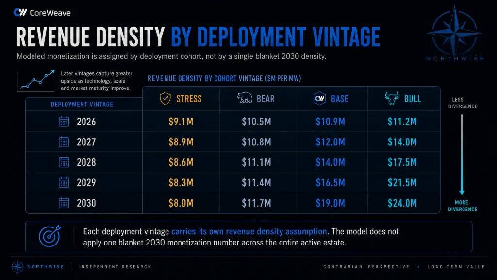
The case for rising revenue density has four components, only one of which is pricing.

The first is physical: a megawatt of 2030 hardware performs substantially more computation than a megawatt of 2026 hardware, since accelerator generations improve compute per watt and rack densities continue to climb. A customer buying throughput will pay more for the same electrical footprint. The second is service attachment, where storage, networking, orchestration, observability, and managed operations all generate revenue against the same megawatt. The third is workload mix, as inference and production serving add continuous utilization alongside project-based training.

The fourth is platform maturity. Weights & Biases, cluster management tooling, and integrated developer workflows lift what a customer will pay for the same underlying silicon, and they raise the switching cost of leaving.

None of that reprices the existing fleet, which is the discipline most models abandon at exactly this point. A contract signed in 2026 for capacity delivered in 2027 runs on 2026 terms, 2026 hardware, and 2026 service scope until it expires. Applying a 2030 density assumption to a 2027 cohort is the single most effective way to manufacture a valuation that cannot happen.

Our model therefore assigns density by deployment vintage and holds each cohort at its own economics.

The scenarios differ on who captures the improvement rather than on whether the improvement happens. Stress assumes newer hardware gets cheaper for the customer faster than CoreWeave develops higher-value services, so density falls even as compute per megawatt rises. Bear assumes real technological progress with weak value capture, which is what a competitive market looks like once supply arrives. Base assumes meaningful monetization from density, inference, utilization, storage, networking, and orchestration, and bull assumes CoreWeave becomes a genuine full-stack platform capturing a share of next-generation compute productivity.

12. The Fleet, Not the Newest GPU

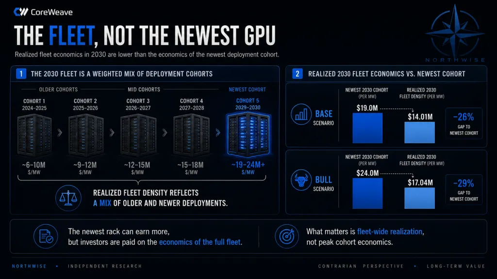
Vintage discipline produces its payoff here, in the gap between the newest cohort and the fleet that actually generates the revenue.

The $19.0 million base and $24.0 million bull figures from the vintage table apply to capacity deployed during 2030 and to nothing else. Weighted across a fleet built over 5 years, base realizes $14.01 million and bull realizes $17.04 million. The difference between the marginal number and the realized number is roughly $5 million per megawatt in base, which across 6.53 GW is more than $32 billion of annual revenue.

Any model quoting a single revenue-per-megawatt figure for 2030 is either describing the newest cohort or the whole fleet, and the two answers differ by 36%.

13. Recognized Revenue Through 2030

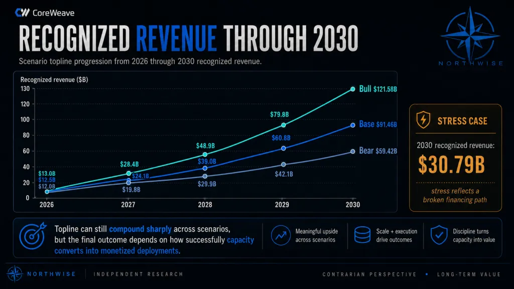
Multiplying average billable capacity by realized vintage-weighted density produces the revenue trajectory.

Stress terminal revenue is 3,520 MW at $8.75 million, or $30.79 billion.

Hold the bear column against the 2025 result of $5.131 billion for a moment. Our downside operating case has CoreWeave growing revenue more than 11 times in 5 years, which describes an outstanding business by any conventional standard. The equity outcome attached to that scenario is examined in the premium sections and it is not good.

That disconnection is the entire thesis, and everything from here forward explains why it exists.

Part IV: The Cost of Building the Cloud

14. What One Megawatt Costs

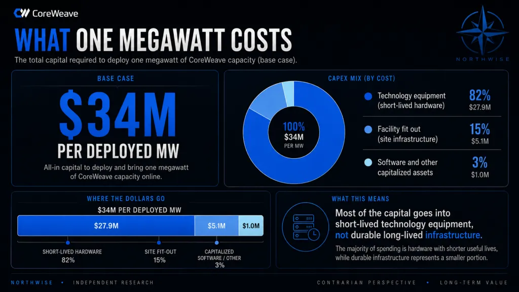
Approximately $34 million buys one deployed megawatt in the base case.

That figure combines technology equipment, networking, storage, facility fit-out, software, installation, and the associated deployment capital required to make the megawatt billable. It is not a landlord-style cost per physical megawatt, since CoreWeave does not build the shell or the substation. Comparing it to an owner-operator's fully loaded build cost is comparing two different products.

The composition explains most of the company's financial behavior.

Roughly 4 dollars in 5 buy an asset with a 6-year accounting life and a shorter competitive one. A company whose capital is 82% weighted toward equipment will show enormous depreciation, will need continuous access to hardware financing, and will face a replacement decision on a cycle far faster than any traditional infrastructure business.

15. Rent Before Revenue

Rent is the cost that arrives first and cares least about what CoreWeave decides afterward.

Our terminal assumption is $2.00 million of annual rent per externally leased megawatt in base and bull, $2.20 million in bear, and an elevated figure in stress. The disclosed 525 MW arrangement supports that level directly: $18.7 billion to $19.6 billion of contractual rent across 16 years works out to roughly $2.28 million per megawatt per year. At scale, every gigawatt of externally leased capacity carries approximately $2 billion of annual rent before a dollar of revenue arrives.

Bull does not receive an automatic rent discount for being larger. Persistent power scarcity strengthens landlord economics alongside CoreWeave's, and a tenant negotiating for capacity in a constrained market has less leverage than one negotiating during a glut. Assuming that operational success translates into cheaper rent would give the bull case two favorable outcomes from one variable.

Our cost structure separates external fixed rent, electricity, non-power facility operations, and compute and cloud operating costs into distinct lines. One correction deserves explicit mention for anyone rebuilding this model. Economic capital charges on controlled campuses are not counted as an EBITDA expense and then counted again through depreciation and interest.

16. The Capex Machine

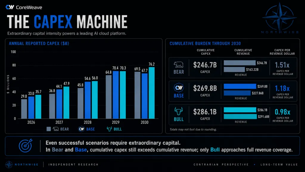
Building 6.5 GW of additional active power consumes roughly $270 billion.

Two features of that table deserve attention. Bear spends $246.7 billion, which is only 8% less than base, since most of the commitment is made before the weaker outcome becomes visible. And bull spends more in 2030 than base does, since a company still accelerating at the terminal date has not yet slowed its deployment.

The base column separates into growth and refresh, and the split changes materially across the period.

One comparison does more work than any paragraph in this section. Set cumulative capital expenditure against cumulative revenue across the same 5 years.

In the base case CoreWeave spends approximately $42 billion more building the platform than the platform earns in revenue over the entire forecast period. In bear the gap widens to $83 billion. Only in bull does cumulative revenue finally catch cumulative investment, and it does so in the final year.

That is the defining financial characteristic of this business, and it is why the capital structure decides the equity outcome rather than the demand environment. A company outspending its own revenue for 5 consecutive years has to raise the difference from somebody, and whoever provides it gets paid before shareholders do.

Refresh spending rises from 5% of capital in 2026 to 22% in 2030 as the earliest cohorts age. That $15 billion figure in 2030 is not the normalized maintenance assumption we use for valuation, which section 20 addresses separately. It is what CoreWeave will actually spend that year on a fleet whose average age is still well under the accounting life.

17. Customer Prepayments Are Not Free Cash Flow

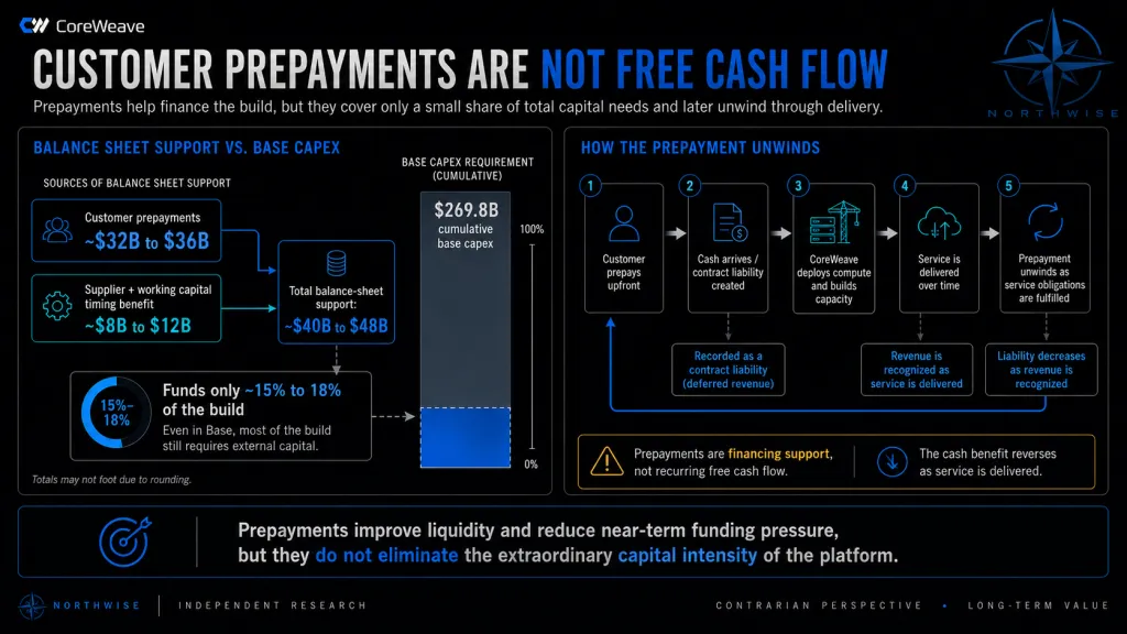
CoreWeave's customer contracts have historically included material prepayments, and its delayed-draw facilities are collateralized by underlying assets and contractual cash flows from generally investment-grade counterparties.

Our base model assumes roughly $32 billion to $36 billion of cumulative customer prepayments through 2030, alongside $8 billion to $12 billion of supplier and working-capital timing benefit, for approximately $40 billion to $48 billion of combined balance-sheet support. Against $269.8 billion of cumulative capital expenditure, that funds roughly 15% to 18% of the build.

The mechanism is genuinely valuable. A prepayment reduces the capital CoreWeave must raise, carries no contractual interest, improves project returns, and provides cancellation protection that a lender would charge for. During a shortage, customers will pay it.

Two things follow that get forgotten routinely. Prepayments are financing, not earnings, and they unwind through service delivery as later invoices are reduced against the prepaid balance. Both phases belong to the same contract, and treating the inflow as cash generation while treating the unwind as a working-capital surprise misreads the arrangement in both directions.

The second point is that prepayment terms are a scarcity artifact. Customers accept them when the alternative is waiting, and the terms compress when it stops being the alternative.

Part V: EBITDA Is Not the Finish Line

18. Why 60% Adjusted EBITDA Can Still Be Expensive

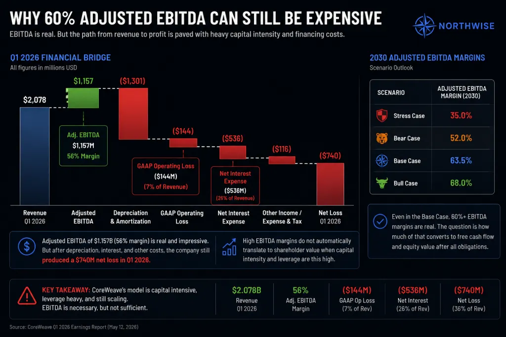
CoreWeave's first quarter of 2026 is the cleanest illustration available of the gap this section addresses.

Revenue was $2.078 billion, adjusted EBITDA was $1.157 billion at a 56% margin, and the company reported a GAAP operating loss of $144 million, net interest expense of $536 million, and a net loss of $740 million. A 56% adjusted margin produced a nine-figure quarterly loss. The 2025 full year showed the same shape more gently, with $3.093 billion of adjusted EBITDA against $2.454 billion of depreciation and amortization.

Adjusted EBITDA is a real measure of operating performance and an incomplete one for a business whose cost of goods sold is a machine it has to buy again. The metric excludes the depreciation of the asset generating the revenue, the interest on the debt that bought it, the principal repayment on that debt, and the capital required to replace it before the contracts renew. In a software business those exclusions are minor. In a compute business they are most of the economics.

Our terminal margin assumptions reflect a larger and more capable organization than the one operating today.

Note that margins do not expand in proportion to revenue density. Managed cloud, inference serving, and software raise what a customer pays for a megawatt while adding platform engineers, site reliability engineers, security staff, solutions architects, and support organizations. The premium creates value only where incremental revenue exceeds the incremental cost of delivering it, which is why our base case lifts density by 74% between the 2026 and 2030 vintages and lifts margin by 7.5 points.

Applying these margins produces the terminal operating result.

19. The Depreciation Wall

Depreciation is where an extraordinary EBITDA figure meets the asset that produced it.

One methodological point governs the schedule. Depreciation begins when an asset is placed into service, not when the capital is paid, and an earlier version of this model overstated the charge by placing too much forward procurement into service immediately. That correction lowered terminal depreciation meaningfully and has been carried through every scenario.

The bear row is the one to sit with. A company generating $30.9 billion of adjusted EBITDA is consuming $36.0 billion of accounting value from its asset base in the same year, which produces a GAAP operating loss on a fleet running near capacity under contracted revenue.

Accounting life and economic life answer different questions, and the model does not assume an accelerator becomes worthless in year 6. The realistic path is a cascade: frontier training first, then enterprise training, then production inference, then fine-tuning and batch work, then retirement when power and support costs exceed what the hardware earns. That sequence extends economic life well past the first contract and reduces dependence on resale assumptions nobody has tested through a full architecture cycle.

The cascade works at declining economics at every step. Useful is not the same as premium, and our model prices later-life hardware accordingly.

20. The Replacement Reserve

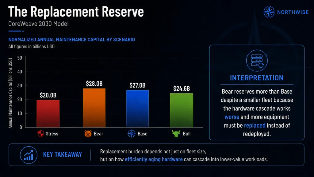
The 2030 fleet is young, which makes the reported refresh figure a poor guide to the sustaining cost of the platform.

Most base-case capacity installs between 2028 and 2030, so a large share of the accelerators generating 2030 revenue are in their first or second year of service. Reported refresh spending of $15 billion in base reflects the replacement of the 2026 and 2027 cohorts and nothing beyond that. Running the platform indefinitely costs considerably more.

Bear carries a higher reserve than base despite operating a smaller fleet, which is deliberate. In bear, the cascade functions poorly: older accelerators find weaker inference demand, second-contract pricing compresses, and a larger share of the fleet has to be replaced instead of redeployed. Base assumes a service layer and workload mix that extend economic life, so the same physical replacement burden spreads across more years and more revenue.

Bull carries the lowest reserve against the largest fleet for the same reason, amplified by better density and stronger residual economics. A megawatt earning $17 million supports its own replacement more comfortably than one earning $11 million, whatever the hardware costs.

These figures are deliberately more conservative than extending the reported 2030 refresh program forward. We would rather understate terminal cash generation than publish a number that quietly assumes CoreWeave never has to buy its fleet a second time.

21. What EBITDA Leaves for the Asset

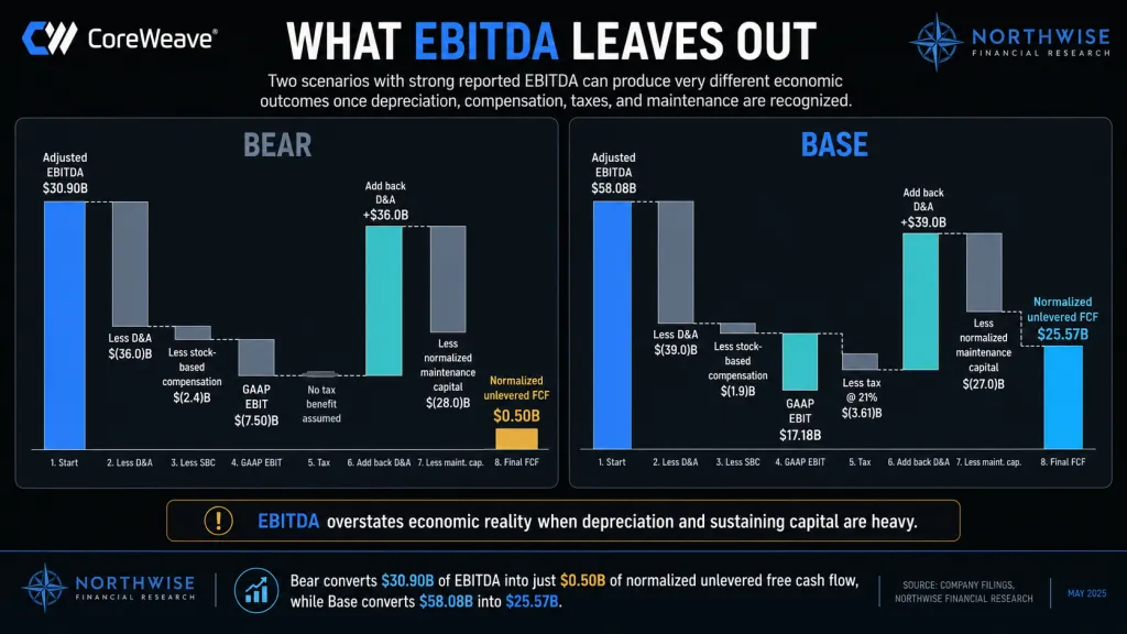
Stock-based compensation is the last item before the operating result becomes an accounting one, and the model does not treat it as free.

Compensation paid in shares appears twice in our framework: once as an expense in GAAP operating income and again through the share count that divides the final equity value. Counting it in neither place, which is the industry convention, produces a valuation that charges nobody for the labor.

Bear carries the highest compensation charge in the model at $2.4 billion despite running the smallest surviving platform. Delivering a given dollar value of compensation requires more shares when the equity price is depressed, and retaining engineers becomes more expensive precisely when the stock has disappointed them. The charge is a symptom of the scenario, not a cause of it.

From EBIT we normalize to unlevered free cash flow, taxing positive operating income at 21%, adding back depreciation, and subtracting the normalized maintenance reserve. Negative operating income receives no artificial tax benefit.

The bear result is the most important single figure in the free portion of this report. CoreWeave can build a $59 billion revenue business generating more than $30 billion of adjusted EBITDA and produce essentially zero normalized economic free cash flow. Nothing has gone wrong operationally in that scenario. The company simply captured less of the value it created than the capital structure required.

Part VI: The Financing Stack

22. Leverage Is Not the Bear Case

High leverage and capital-structure failure are different conditions, and conflating them produces bad analysis in both directions.

CoreWeave funds itself through six overlapping channels. Delayed-draw term loans and project finance sit at the base, secured by assets and pledged contractual cash flows, with $11.8 billion outstanding at March 31 across the delayed-draw facilities alone. OEM and equipment financing funds hardware directly against collateral that decays on a schedule set by the vendor's roadmap. Unsecured corporate notes fund the platform layer that cannot be attached to any single contract, which makes them the most expensive money in the stack.

Convertibles sit above that, equity issuance above that, and customer prepayments beside all of it. The company has stated directly that future expansion will continue to depend on debt, equity, delayed-draw facilities, OEM financing, and balance-sheet cash.

Terminal debt varies with scenario in a way that rewards careful reading.

Bear carries more absolute debt than base while operating a smaller platform. Weaker project economics require more external funding per megawatt, a weaker equity price makes issuance more painful, and the shortfall lands on the credit side. Bull carries the least debt against the largest asset base, since strong operations generate internal cash and command better terms.

We deliberately declined to lower base or bull debt after raising terminal revenue density. Allowing stronger operations to simultaneously produce more revenue, better margins, and a cleaner balance sheet would let one favorable assumption pay three times.

23. What the Debt Actually Costs

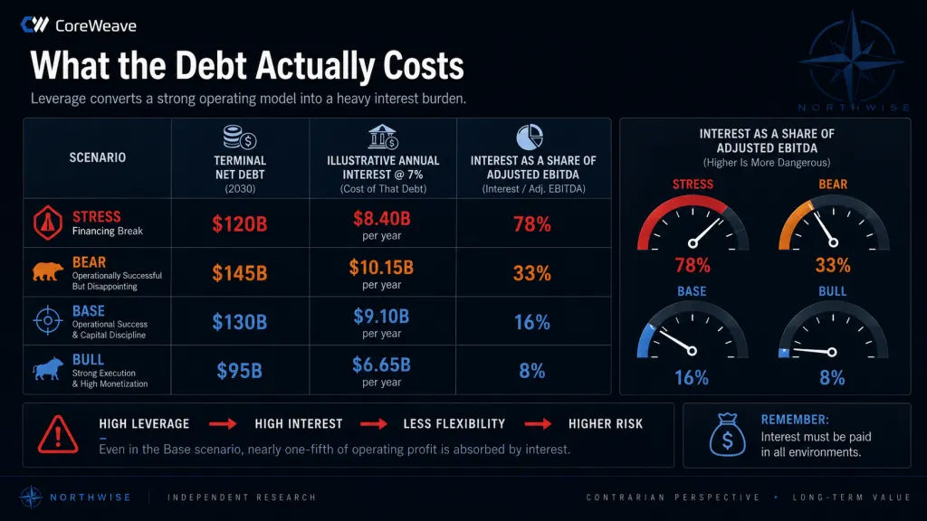
Our valuation framework works in unlevered terms and deducts net debt at the enterprise level, so interest never appears in the free cash flow lines. That is methodologically correct and it hides something a shareholder should see.

CoreWeave reported $536 million of net interest expense in the first quarter of 2026 against $25.1 billion of principal debt, which annualizes to a blended cost near 8.5%. The marginal cost looks better than the historical blend, with the DDTL 4.0 facility pricing at SOFR plus 2.25% floating and roughly 5.9% fixed. The table below applies an illustrative 7% to terminal net debt as a diagnostic, not as a model input.

Interest alone consumes 78 cents of every EBITDA dollar in stress and 8 cents in bull. Stack depreciation on top and the levered accounting picture separates the scenarios more sharply than any operating metric does.

Bear generates $30.9 billion of adjusted EBITDA and remains roughly $15 billion underwater on a levered pre-tax basis. Base clears the bar by less than $10 billion on $91 billion of revenue. Those two rows are the reason the equity outcomes in Part XII diverge as violently as they do.

Rent behaves differently and deserves separating. Approximately $2 million per leased megawatt per year already sits inside the EBITDA margin as an operating cost, which means the base case is absorbing roughly $15 billion of annual rent before the interest above is charged. A reader adding rent to this table would be counting it twice.

24. Convertible Capital

Convertible notes are the most commonly mishandled item in neocloud valuation, and the error runs in a consistent direction.

CoreWeave carries $6.588 billion of convertible principal in our terminal model. Investors frequently treat the instrument as equity, which understates the downside: until conversion or settlement it remains a senior claim, and a stock sitting below the conversion threshold near maturity forces repayment, refinancing, or issuance at weak prices. In a poor outcome it behaves like debt and in a strong one like dilution, and shareholders pay one of the two.

Our treatment is symmetric. Where conversion is economically expected, we remove the $6.588 billion of principal from net debt and add the residual dilution that survives capped-call protection. We never subtract the debt and add the full underlying share count in the same calculation, which is the error that quietly inflates a large share of published price targets.

Residual dilution after capped calls is approximately 16.29 million shares in base and 44.48 million in bull. Bull carries more residual dilution than base, since a higher share price pushes further above the cap where the hedge stops offsetting.

25. The Lease-Adjusted Balance Sheet

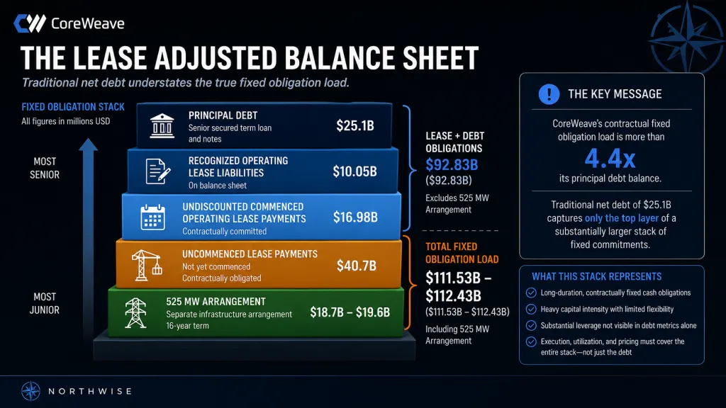
Conventional net debt understates CoreWeave's fixed obligations by a wide margin.

The March 2026 disclosures show $10.05 billion of recognized operating lease liabilities, $16.98 billion of undiscounted commenced operating lease payments, and $40.7 billion of uncommenced lease payments, before the separate 525 MW arrangement carrying $18.7 billion to $19.6 billion over 16 years. Recognized liabilities capture a small fraction of the total commitment, since accounting recognition begins when a lease commences and CoreWeave has signed for capacity that landlords have not yet delivered.

For any credit or downside analysis, rent belongs alongside interest as a contractual, non-discretionary, long-duration payment. A company with $25.1 billion of principal debt and something approaching $77 billion of contractual rent is more levered than its debt balance suggests, and the rent has a longer duration than most of the debt.

The obligations also behave differently under stress. Debt can sometimes be restructured, extended, or exchanged, and a data-center lease in a market where powered capacity is scarce gives the landlord considerable leverage in any renegotiation.

26. The Denominator Problem

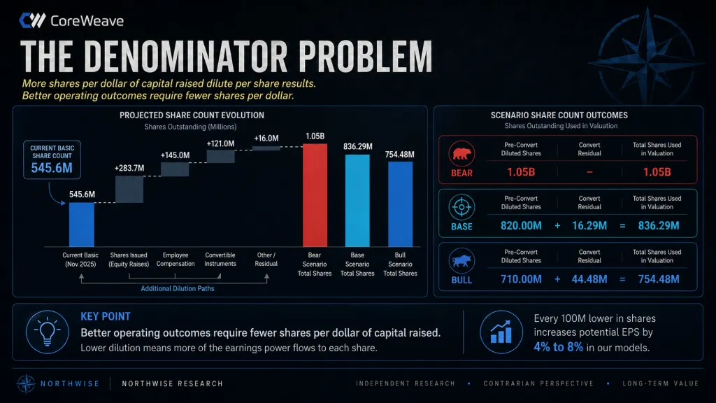
CoreWeave's opportunity is measured in gigawatts and its outcome is measured per share.

The basic share count stood at approximately 545.6 million in April 2026. Our model then layers existing options, restricted awards, RSUs, future employee grants, future equity issuance, warrants, and convertible dilution across the forecast period.

The relationship between execution and dilution is the least intuitive part of the model and the most important. Better outcomes require fewer shares per dollar of capital raised, since a stronger equity price, more customer funding, better debt terms, and higher internal cash generation all reduce how much equity has to be sold. Base issues roughly 274 million shares beyond the current count. Bear issues more than 500 million while building a smaller company.

That is the mechanism by which a good operating result becomes a poor investment result. Enterprise value grows in every scenario except stress, and the claim attached to each existing share does not.

27. The Flywheel in Reverse

The route to stress does not require demand to disappear, which is what makes it worth modeling seriously.

The sequence starts with delay. Landlord delivery slips, commissioning takes longer than planned, or acceptance on a large cluster is deferred, and revenue arrives later than the rent and debt service it was supposed to cover. Fixed obligations do not move when schedules do.

The shortfall then reaches the equity price, which raises the cost of the next capital raise, which forces either more dilution or more debt at worse terms. Higher leverage tightens covenants and reduces the appetite of the lenders whose delayed-draw commitments fund the next deployment. Slower deployment means slower revenue, and the loop closes.

Two features make this path more plausible than it looks from a chart of the backlog. CoreWeave does not control the construction schedule for the buildings it occupies, and its 82% equipment-weighted capital base means the collateral securing much of its debt declines in value on a vendor's product cadence.

Stress in our framework is a financing event rather than a demand event. The company still reaches 4.2 GW and $30.79 billion of revenue, since the capital was committed and the leases were signed years before the difficulty arrived.

Part VII: Competition and the Migrating Bottleneck

28. CoreWeave Against Its Peers

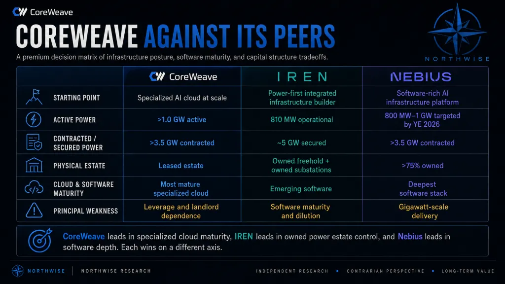
CoreWeave, IREN, and Nebius are building the same platform from three different starting points, which makes the comparison unusually clarifying.

The cost of CoreWeave's choice shows up in the unit economics. Our IREN work puts the infrastructure layer, meaning land through substation and shell, at roughly $14.5 million per gross megawatt to own. CoreWeave pays approximately $2 million per megawatt per year to rent the equivalent function, which across a 16-year lease term is a multiple of the ownership cost. The measurement bases are not perfectly comparable, and the direction is unambiguous.

What CoreWeave bought with that premium was time and the absence of development risk. IREN spent years on grid studies, interconnection queues, permitting, and transformer procurement before earning a dollar of AI revenue, and CoreWeave skipped all of it to reach 1 GW active first.

The difference reappears when hardware economics deteriorate. IREN can energize a substation and decline to equip the megawatt, which our base case for that company reflects directly with 6.0 GW energized against 4.6 GW equipped. CoreWeave has already committed to rent on capacity it may not want to fill at prevailing terms. The optionality IREN preserves at the cost of speed is the optionality CoreWeave sold to acquire it.

Nebius attacks from the third direction and is the competitor most likely to converge on CoreWeave's revenue density while diverging on financing economics. It reported $390 million of AI Cloud revenue and $1.9 billion of ARR in the first quarter of 2026 against guidance for $7 billion to $9 billion of year-end ARR, and it has moved hard toward owned facilities with a Pennsylvania project of up to 1.2 GW, a 1.2 GW Missouri project, and a 310 MW Finland site. Its platform spans infrastructure, serverless inference, training, production deployment, enterprise security, and developer services.

Nebius is not asset-light in any sense that would make its capital position comfortable. It spent approximately $2.47 billion on property, equipment, and intangibles during a single quarter against 253.9 million shares outstanding, and its expansion increasingly requires debt, convertibles, equity, and customer commitments. All three companies are running the same trade with different collateral.

Where the models genuinely diverge is in what survives 2030. IREN and Nebius will own durable physical layers that outlast several hardware generations. CoreWeave will own contracts, software, customer integrations, and a fleet. Revenue density can converge completely and the terminal asset bases will still look nothing alike.

29. The Bottleneck Moves

Competition in this sector changes shape as the binding constraint migrates, and each migration rewards a different capability.

CoreWeave's strength sits in the fourth and fifth rows, which is a more defensible position than most of its investors appreciate. Standing up a 10,000-accelerator cluster that passes a frontier laboratory's benchmarks on multi-node scaling, networking efficiency, and reliability is a genuine operational capability, and a large share of the industry cannot currently do it well.

The moat is therefore not the chips, since anyone with capital can buy those. It is time to compute, the software layer customers integrate into production workflows, the depth of those integrations, the financing apparatus, and the accumulated competence of an organization that has done this at scale repeatedly. Those advantages are real and they are not permanent.

The rows below CoreWeave's position are where the value migrates next. Enterprise adoption rewards compliance, security posture, sales organization, and workflow integration, and mature competition rewards cost efficiency and switching value. CoreWeave has to climb into those rows before the market finishes passing through the ones where it currently leads.

Part VIII: The Three Clocks

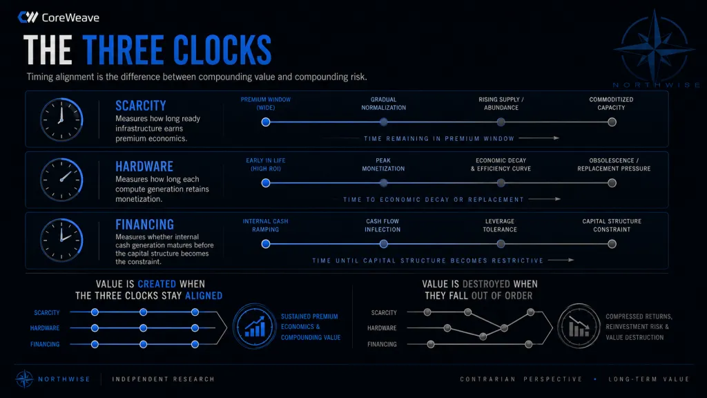
30. Scarcity, Hardware, Financing

Three sequences have to stay aligned for this equity to work, and none of them tells you anything useful in isolation.

The scarcity clock measures how long ready infrastructure commands premium economics. It is currently running slowly in CoreWeave's favor, visible in contract duration, pricing, prepayment terms, and the willingness of investment-grade counterparties to commit years ahead of delivery. It stops when hyperscalers finish internal campuses, competing operators energize comparable sites, and customers gain the experience and the alternatives to negotiate properly.

The hardware clock measures how long each compute generation retains sufficient monetization. Frontier training economics last roughly one to two generations, after which the cascade into enterprise training, inference, and batch work sustains the asset at declining prices. This clock runs on a schedule set by a vendor whose interests do not require CoreWeave's fleet to age gracefully.

The financing clock measures whether operating cash matures before the capital structure becomes the constraint. CoreWeave is currently funding growth with debt, leases, prepayments, and equity, and the question is whether internally generated cash arrives in time to reduce that dependence. Base answers yes with $25.57 billion of normalized unlevered free cash flow in 2030, and bear answers no at $0.50 billion.

Value gets created when capacity arrives before the scarcity clock expires, contracts return capital before the hardware clock weakens, and cash generation matures before the financing clock tightens. Value gets destroyed when they fall out of order.

31. The 2030 Convergence

Our valuation date sits in an awkward place in CoreWeave's own asset cycle, and the terminal multiples reflect that directly.

Several things arrive at once between 2030 and 2032. The earliest large contracts reach renewal, the 2026 through 2028 hardware cohorts require repositioning or replacement, the normalized maintenance burden becomes real spending, project debt amortizes against a fleet whose collateral value has stepped down, and convertible planning begins in earnest.

Each of those is manageable alone. Arriving together, they compete for the same cash in the same window.

The market will not pay the same multiple for $91 billion of revenue arriving with renewals settled, refresh funded, and a stable share count as it will for $91 billion arriving with all three unresolved. That is the real content of the terminal multiple discount applied in the premium sections, and it is a more precise statement than describing the company as risky.

Part IX: The Case Against the Sector

32. The Short Thesis, Stated Properly

The strongest argument against this entire category does not come from people who think AI is a fad. It comes from people who can read a depreciation schedule.

Stated in its own register, it runs roughly as follows. A neocloud is a leveraged rental business on a rapidly depreciating asset, and it is being valued as though it were software. The cost of goods sold in a GPU cloud is the GPU, spread across a 6-year book life that may prove generous, and excluding it from the headline metric converts a marginal business into an apparently exceptional one. Adjusted EBITDA is not a proxy for cash when the asset consuming the cash has to be repurchased before the contracts renew.

The financing compounds the problem, on this view. Capital expenditure is funded by debt, leases, and equity issuance instead of operations, the equity is sold into enthusiasm, and the debt is collateralized by hardware whose resale market has never been tested through a full architecture cycle. Backlog assumes counterparties still exist in year 4 and still want the same terms. Lease obligations that exceed the debt balance sit largely outside the leverage ratios most investors quote.

The circularity is the part that should trouble people most. One vendor supplies the accelerators, invests in the buyers, and books the revenue, while the buyers cite the vendor's participation as validation. That structure has appeared before in telecommunications equipment, and the analogy that fits is not AWS in 2010. It is dark fiber in 1999: real demand, real assets, real technology, and a decade of returns transferred from the builders to the users once supply arrived.

The conclusion follows without requiring AI to disappoint. When capacity catches up, rents fall toward cash cost, the buildings and substations retain value, and the equity does not.

33. Where We Part Company

Large portions of that argument are already inside our model, which is why our bear case carries substantial weight instead of appearing as a rhetorical gesture.

Depreciation is why section 19 shows bear consuming 117% of its adjusted EBITDA in accounting charges. The refusal to apply software multiples is why our terminal enterprise values sit at a fraction of what a comparable-growth software business would command. The untested resale market is why the normalized maintenance reserve exceeds reported refresh spending in every scenario. The bear case, at $59.4 billion of revenue and roughly zero normalized free cash flow, is essentially this argument playing out over 4 years.

We part company on three points. The first is substitutability: the short case treats powered, energized, interconnected capacity as reproducible on roughly the same schedule as chips, and interconnection queues do not behave that way. Foundry capacity, packaging, and yields can all expand, while transmission develops on a timetable set by utilities and regulators.

The second is asset recourse. Fiber in 1999 had no alternative buyer at scale, and a completed gigawatt-class campus with contracted power has several, including the hyperscalers whose internal programs are running behind their own demand.

The third is the software layer. A customer running orchestration, storage, monitoring, and experiment tracking on CoreWeave faces a materially harder migration than one renting bare hardware, and the short case tends to price the second while the company is increasingly selling the first.

The honest synthesis is that the skeptics are describing our bear case with more confidence than we can justify assigning it, and we are describing our base case with more confidence than they can justify rejecting. Both readings start from identical facts. The disagreement is about how long physical scarcity persists and who holds the pen when it ends.

Part X: What Moves the Model

34. The Variables That Decide the Outcome

Our model moves toward the upper scenarios on a specific and observable set of developments.

Revenue density is the largest single lever. Contract expansions at improving pricing, a shift toward direct customer relationships instead of intermediated capacity, monetization of Weights & Biases and inference services, and evidence that second-contract hardware earns more than we assume would each push the density curve higher. Lower sponsor capital per megawatt, whether through larger prepayments, cheaper project debt, or better OEM terms, would reduce dilution and improve per-share value without changing a single operating assumption.

The model moves down on a mirror image of that list. A persistent gap between active and billable capacity signals that the commercial organization has outrun the deployment organization. Pricing compression, shrinking prepayments, expensive renewals, weaker inference demand, landlord rent inflation, growth in unsecured corporate debt, equity issuance at depressed prices, and poor hardware reuse each cost real value, and they tend to arrive together.

Eight metrics carry most of the information, and CoreWeave discloses only some of them.

The confirming signal for base is a small contract growing into a multi-site relationship at stable or improving density. The warning signal is rapid capacity growth alongside flat or falling revenue per billable megawatt.

Part XI: The Four Outcomes

35. Four Versions of the Same Company

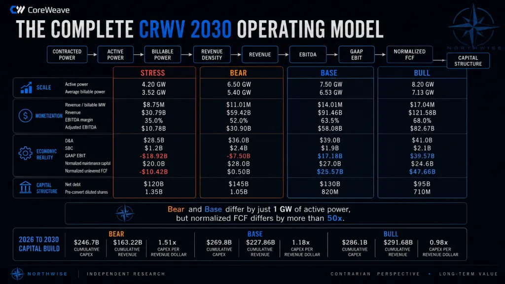
All four scenarios begin with the same demand. They diverge through deployment speed, revenue density, capital efficiency, debt, leases, and dilution.

Stress is a financing event. Delay, cost, or a closed capital window forces a major recapitalization or restructuring, and CoreWeave still reaches 4.2 GW of active power and $30.79 billion of revenue, since the leases were signed and the capital committed years earlier. Adjusted EBITDA of $10.78 billion sits against $28.5 billion of depreciation and $120 billion of net debt, producing negative normalized free cash flow of $10.42 billion and a capital structure that has to be reorganized.

Bear is the scenario every investor in this sector should study most carefully. CoreWeave reaches 6.5 GW, generates $59.42 billion of revenue at a 52% adjusted EBITDA margin, and produces $30.90 billion of adjusted EBITDA. It also carries $36.0 billion of depreciation, $145 billion of net debt, more than 1.05 billion shares, and $0.50 billion of normalized unlevered free cash flow. The company succeeded, the market grew, the contracts were signed, and the value went to landlords, lenders, and new shareholders.

Base has the cloud outrun the capital structure. Active power reaches 7.5 GW, average billable capacity reaches 6.53 GW, realized density reaches $14.01 million, and revenue reaches $91.46 billion at a 63.5% margin. Depreciation of $39.0 billion and stock compensation of $1.9 billion leave $17.18 billion of GAAP operating income, and after tax, depreciation add-back, and a $27.0 billion maintenance reserve, $25.57 billion of normalized unlevered free cash flow.

Bull has the infrastructure lead become a platform. Active power reaches 8.2 GW, realized density reaches $17.04 million, revenue reaches $121.58 billion at a 68% margin, and normalized free cash flow reaches $47.66 billion against the lowest net debt and share count in the model. It requires the scarcity window to stay open long enough for the software and service layer to become the reason customers stay.

Note what separates these outcomes. Bear and base differ by 1.0 GW of active power and roughly $3 million of realized density, and they produce a 51-fold difference in normalized free cash flow.

36. The Complete CRWV Stock Forecast 2030 Model

The full operating picture, with no valuation applied.

Read the D&A row against the adjusted EBITDA row before anything else. Stress and bear both consume more accounting value from their asset base than they generate in adjusted EBITDA, which is how a company can run a full fleet under contracted revenue and still post an operating loss.

37. The Same Model, Per Megawatt

Scale hides quality, so the cleanest test of these four outcomes is to divide every line by the capacity that produced it.

Every row moves in the same direction once capacity is stripped out, which is what a coherent model should produce and what a model built backward from a desired answer usually cannot.

The maintenance row resolves an oddity in the absolute figures. Bear reserves $28.0 billion against base's $27.0 billion while running a smaller fleet, which looks backward until the capacity is divided out. Per megawatt, bear reserves $5.19 million against base's $4.14 million, since a weaker hardware cascade means more of the fleet gets replaced instead of redeployed into inference and batch work. The absolute figures cross over and the underlying assumption never does.

Net debt per megawatt may be the single clearest expression of this thesis. Stress carries $34.09 million of net debt against each billable megawatt and bull carries $13.32 million, a spread of 2.6 times against platforms whose physical scale differs by roughly 2 times. The scenarios diverge less on how much gets built than on how it gets paid for.

Depreciation per megawatt tells the capital-efficiency story directly, falling from $8.10 million in stress to $5.75 million in bull. Better outcomes are not buying cheaper hardware. They are converting the same deployment into more billable capacity and more revenue per unit of capital, which is what deployment speed, acceptance discipline, and service attachment actually purchase.

The bottom row carries the conclusion. A megawatt in bear produces $90,000 of normalized free cash flow and a megawatt in base produces $3.92 million, against revenue that differs by only 27%. Everything between those two rows is cost structure, capital intensity, and financing.

38. What Has to Be True

Each outcome reduces to a handful of conditions that can be checked against reported results instead of argued about.

Base requires four things to hold together. Active power has to reach roughly 2.85 GW by the end of 2027 and 4.10 GW by the end of 2028, which is a construction and landlord-delivery test more than a demand test. Realized fleet density has to climb from roughly $10.9 million toward $14.01 million, which requires service attachment and inference monetization to outpace pricing compression. And diluted shares have to stay near 836 million, which requires customer prepayments and project debt to keep funding the large majority of each deployment.

Bear requires only that the first condition hold while the second and third fail. Capacity arrives close to schedule, demand shows up, contracts get signed, and density stalls near $11 million while the share count runs past 1.0 billion and net debt reaches $145 billion. Nothing in that sequence requires a mistake, a scandal, or a downturn. It requires ordinary competition arriving on an ordinary timetable.

Bull requires all four base conditions plus two more. Density has to reach $17.04 million realized across the fleet, which means the software and service layer becomes the reason customers stay instead of a convenience they tolerate. And net debt has to fall to $95 billion while the platform grows to 8.20 GW, which requires internally generated cash to displace external funding before the terminal date.

Stress requires none of the above to fail on the demand side. It requires the timing to break: landlord delivery slipping, acceptance deferring, or the capital window closing while $25 billion of debt, $77 billion of contractual rent, and a partially completed build all continue on their own schedules.

39. What We Reconstructed and What CoreWeave Reported

A model is only as trustworthy as its inputs, so it is worth separating what the company told us from what we built ourselves.

CoreWeave does not disclose contract-level megawatts, customer concentration by revenue, project-level capital expenditure, second-contract pricing, hardware residual values, or the lag between energization and billing. Those are precisely the variables that determine per-share returns, which forces indirect estimation of the things that matter most.

The pattern to notice is that the left column gets softer as the model moves right in time. The 2026 column is anchored to guidance and reported results. The 2030 column is a Northwise construction, disciplined by arithmetic and constrained by disclosure, and still a construction.

A reader who wants to attack this model should start with revenue density by vintage and the normalized maintenance reserve. Those two inputs carry more of the outcome than any other pair, and neither has a company-reported analogue to check against.

Continue With Northwise Premium

The operating model is now complete, and everything to this point is arithmetic a careful reader can verify or dispute. CoreWeave can reach 2030 as a distressed financing structure, a massive but economically disappointing cloud, a dominant independent AI platform, or one of the most valuable infrastructure businesses in technology. All four paths begin from demand that already exists and contracts that are already signed, and they diverge through deployment, revenue density, capital efficiency, debt, leases, and dilution.

What follows is judgment, and it answers the only question that reaches a shareholder. What is each of these four outcomes actually worth per share, how likely is each one, and what price today compensates an investor for owning the whole distribution?

Northwise Premium continues with our scenario multiples, 2030 price targets for all four outcomes, the stress recovery tree, probability weighting, the enterprise-value-to-shareholder waterfall, the full present-value ladder, entry and exit zones, and the sensitivities that move the target most.